NOTE: This part requires some basic understanding of calculus.

These are just my solutions of the book Reinforcement Learning: An Introduction, all the credit for book goes to the authors and other contributors. Complete notes can be found here. If there are any problems with the solutions or you have some ideas ping me at bonde.yash97@gmail.com.

Blackjack approximate state value 5.1 - 5.2

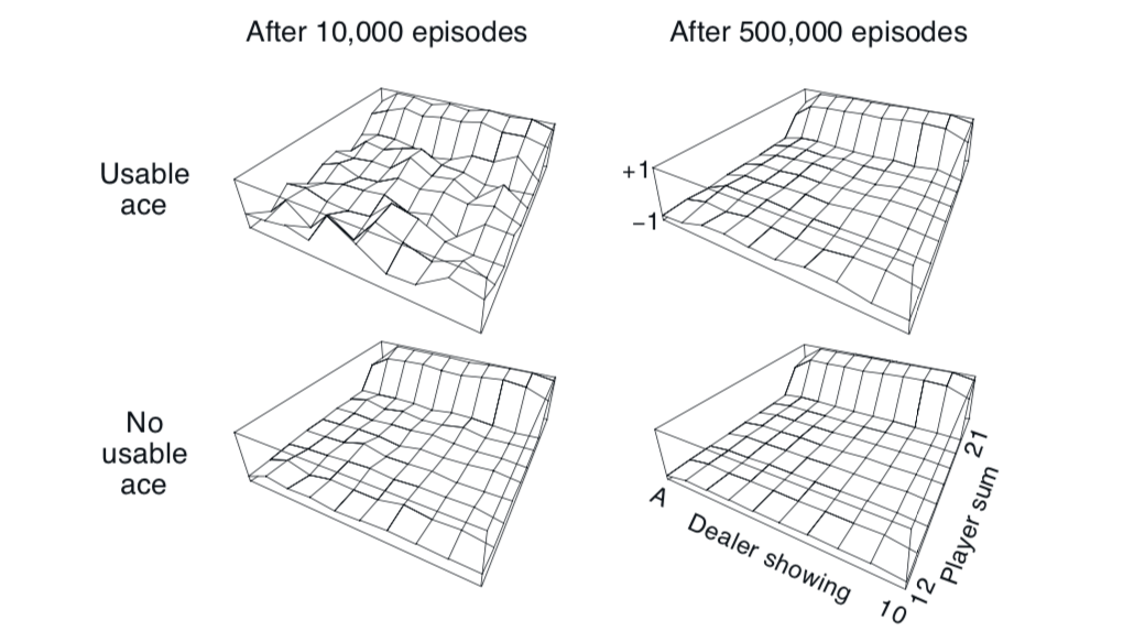
5.1 Estimate Values

The value function jumps up for the last two rows in the rear because the value of the state at that moment is very high due to the sum of cards being in $20-21$ range. The dropoff occurs in the whole last row in the left because the dealer has shown an ace which can either be used as a $1$ or $11$, thus it's confidence of victory is low. The frontmost values are higher in the upper diagrams as having a usable ace in the start is very beneficial.

5.2 Every-visit MC

With every visit MC the training cycles would be quicker as the average would be calculated over a larger reward base with discounts. But we are given that discount factor $\gamma = 1$ for this game and thus there will be no difference in the ETMC and FTMC in this game.

5.4 Improvements to MS-ES pseudo code

We need to add code for incremental averaging which gives us the following equation and it needs to be replaced in the pseudocode

$Q(S_t,A_t) \leftarrow Q(S_t, A_t) + \frac{1}{N(S_t, A_t)}(G - Q(S_t, A_t))$

Also note that the given pseudo code is first visit MC.

5.5 EV-MC and FV-MC estimated value

Looking at the algorithm for first visit we can see that $V_{FC} = +1$ and breaking out a quick script for every-visit we get value $+5.5$.

quick code

5.6 $Q(s,a)$ Value

$V(s) \doteq \frac{\sum_{t\in J(s)}\rho_{t:T(t) - 1}G_t}{\sum_{t\in J(s)}\rho_{t:T(t) - 1}}$

The only change is that instead of counting the state visit we count the state, action visit i.e. $J(s) \rightarrow J(s,a)$

$Q(s,a) \doteq \frac{\sum_{t\in J(s,a)}\rho_{t:T(t) - 1}G_t}{\sum_{t\in J(s,a)}\rho_{t:T(t) - 1}}$

5.7 MSE increases

In the plot for Example 5.4 the error over all decreases but weighted sampling shows a slight rise and then decreases, question is why does this happen?

5.8 Why the jump?

In the plot for Example 5.4 the weight sampling increases and then decreases. This can happen because the value of $\rho$ is large, i.e. the bias is high. Though as the episodes progress the average reduces and so does the bias.

5.9 Change algorithm for incremental implementation

The simple change is the removal of $Returns$ list and getting value of $V(s)$ as

$V(s) \leftarrow V(s) + \frac{1}{N(s)}(G_t - V(s))$

5.10 Derive weight update rule

There are a few things here that $C_n$ represents the cumulative weight till now such that $C_{n+1} = C_n + W_{n+1}$

$V_n = \frac{\sum_{k=1}^{n-1}W_kG_k}{\sum_{k=1}^{n-1}W_k}$

$V_{n+1} = \frac{\sum_{k=1}^{n}W_kG_k}{\sum_{k=1}^{n}W_k}$

$= \frac{1}{W_n + \sum_{k=1}^{n-1}W_k}\big(W_nG_n + \sum_{k=1}^{n-1}W_kG_k \big)$

$= \frac{W_nG_n}{C_n} + \frac{\sum_{k=1}^{n-1}W_kG_k}{C_n}$

$= \frac{W_nG_n}{C_n} + \frac{\sum_{k=1}^{n}W_k}{C_n}V_n$

$= \frac{W_nG_n}{C_n} + \frac{C_n - W_n}{C_n}V_n$

$V_{n+1} = V_n + \frac{W_n}{C_n}(G_n - V_n)$

5.11 Why off-policy MC control removes $\pi(a|s)$

Since $W$ is only allowed to change if $A_t = \pi(S_t)$ and $\pi$ being deterministic we can say that we are safe to $\pi(A_t|S_t) = 1$.